背景#

上次学习了 Radiometry&Monte Carlo Integration 的理论知识，现在觉得自己很强，想学习一下怎么将理论应用到实践中了，你准备在你第一次实现的那个最简单的渲染器上进行扩展，并加入一些新的材质、和优化方法，并且进一步理解上次代码中不懂得一些问题

剧情我是真的编不下去了，相信没什么人喜欢看这个剧情，先不写剧情了，有时间再补吧！

The Lambertian Diffuse Model#

在 Re0:0x02 中我们给出了 BRDF 的定义，但是那只是定义式是没办法用于真正计算的，所以我们需要对真实的材质在我们的定义式下进行建模，通过建模后的式子才适合用于计算。

接下来我们看一个最最简单的 BRDF 模型，就是 Lambertian Diffuse Model , 这是一个漫反射材质模型，顾名思义专门用于建模漫反射材质。

在 Re0:0x01 中我们提到这个模型，其中的代码直接给出了类似下面的代码，现在回过头来看其实不是很合适，因为没有说明 Lambertian 漫反射的 BRDF 是怎么推导的，并且引入了微表面模型，其实那个时候没必要引入微表面模型的，从中可以看到我以前对知识的理解也是非常的浅薄

1
class Material {
2
public:
3
    ...
4

5
    Vec3 eval() const
6
    {
7
        return albedo_ / (3.141592653589793);
8
    }
9

10
private:
11
    Vec3 albedo_{};
12
};

方向半球反射率#

在推导 Lambertian Diffuse Model 的 BRDF 之前我们先介绍一个概念 方向半球反射率 $\rho_{hd}(\omega_i)$ ，它表示对于给定的入射方向 $\omega_i$ ，有多少比例的入射能量被反射到整个半球

\rho_{hd}(\omega_i) = \int_{\mathcal{H}^2(\mathbf{n}) }f_r(p,\omega_i, \omega_o)\cos\theta_o d\omega_o

工程上这就是材质的”反射率”参数，通常用一个 RGB 颜色来表示
它常常被用于验证 BRDF 的能量守恒，即反射的能量不能超过入射的能量

L_o = \rho_{hd} L_i \qquad 0 \le \rho_{hd} \le 1

推导#

好了现在我们开始正式的推导一下 Lambertian Diffuse Model 的 BRDF

Lambertian Diffuse Model 假设

在光线打到漫反射材质上这个光会被均匀的散射到半球的所有方向，或者说是漫反射材质是一种无论观察者从哪个角度看，表面看起来都一样亮的材质

这个假设说明了出射光是一个恒定的常数(因为表面看起来都一样亮)，并且出射光与观察者的角度(出射方向)无关(因为无论观察者从哪个角度看)

我们再来看渲染方程，假设材质不会自发光：

L_o(p, \omega_o) = \int_{\mathcal{H}^2(\mathbf{n}) } f_r(p,\omega_i, \omega_o) L_i(p,\omega_i) \cos\theta_i d\omega_i

很显然标准的渲染方程的 $L_o$ 与出射方向有关，而被积函数中只有 $f_r$ 是与出射方向有关的，而我们要满足假设让 $f_r$ 与出射方向无关

f_r(p,\omega_i, \omega_o) = f_r(p,\omega_i)

需要注意的一点是，在图形学中我们一般默认假设 $f_r(p,\omega_i) = k$ 是一个常数，即我们新增加了一个假设：漫反射材质是各项同性的，但是现实是漫反射材质也可以是各项异性的，但是在图形学中使用各项同性的 Lambertian Diffuse Model 一般就够了，关于什么是各项同性和各向异性材质的可以去自己搜搜，未来我们会讲

所以有

f_r(p,\omega_i) = k

现在我们的渲染方程变为

L_o(p) = k \int_{\mathcal{H}^2(\mathbf{n}) } L_i(p,\omega_i) \cos\theta_i d\omega_i

而根据 Lambertian Diffuse Model 假设 $L_o$ 是一个恒定的常数，注意到如果 $L_i(p,\omega_i)$ 是一个常数可以提到积分外面去,那么剩下的部分就是带余弦权重的半球积分，而对半球得积分为 $\pi$ 。

而我们又知道BRDF 是材质的固有属性与场景无关，所以我们可以构造一个最简单的场景来把它求出来。

我们可以这么构造：以被积微元点为球心放置一个均匀发光的半球，入射 Radiance 恒为常数，即 $L_i$ 为常数。

Q&A:

为什么可以随便构造场景？因为 BRDF 是材质固有属性，跟光照无关，我选什么场景都行，那我选一个最简单的

最简单的是什么？ $L_i$ 处处相等且方向无关的场景

这个时候我们的渲染方程变成

L_o = k L_i \int_{\mathcal{H}^2(\mathbf{n}) } \cos\theta_i d\omega_i = k L_i \pi

而根据方向半球反射率提到的保证能量守恒

L_o = \rho_{hd} L_i \qquad 0 \le \rho_{hd} \le 1

我们联立这两个方程

\left\{\begin{matrix} L_o = \rho_{hd} L_i & 0 \le \rho_{hd} \le 1 \\ L_o = \pi k L_i & \end{matrix}\right.

最后解得

k = \frac{\rho_{hd}}{\pi}

即 Lambertian Diffuse Model 为

f_r = k = \frac{\rho_{hd}}{\pi}

其中 $\rho_{hd}$ 为材质的反射率所以你能看到代码中

1
 return  albedo_ / (3.141592653589793);

而 $k_d$ 只是一个比例系数，后面我们会提到

Importance Sampling of the Lambertian Diffuse Model#

我们看 Re0:0x01 中 Material.h 中的 pdf 代码

1
double pdf(const Vec3& wi, const Vec3& wo, const Vec3& normal)
2
    {
3
        const double cosThetaI = dot(normal, wi);
4
        const double cosThetaO = dot(normal, wo);
5

6
        if (cosThetaI <= 0.0 || cosThetaO <= 0.0) {
7
            return 0.0;
8
        }
9

10
        return 1.0 / (2.0 * constants::PI);
11
    }

这里使用的是均匀采样对应的 pdf，即

p(x) = \frac{1}{2\pi}

而我们在 Re0:0x02 中学习过重要性采样，当选择一个 pdf 它的形状和分子形状类似时方差就会缩小

我们先回顾一下蒙特卡洛积分

\hat{L}_o(p, \omega_o)=\frac{1}{N}\sum_{i=1}^N\frac{f_r(p,\omega_i,\omega_o)L_i(p,\omega_i)\cos \theta_i}{p(\omega_i)}

我们将其写为 Lambertian Diffuse Model 的形式

\hat{L}_o(p, \omega_o)=\frac{1}{N}\sum_{i=1}^N\frac{(\frac{\rho}{\pi})L_i(p,\omega_i)\cos \theta_i}{p(\omega_i)}

我们将其变形为

\hat{L}_o(p, \omega_o)=\frac{1}{N}\sum_{i=1}^N\frac{\frac{\cos \theta_i}{\pi}}{p(\omega_i)} \rho L_i(p,\omega_i)

当我们令 $p(\omega_i) = \frac{\cos \theta_i}{\pi}$ 的时候这个分式就直接变成 1 了，这就是我我们的目标

而学过概率论的都知道一个合法的 pdf 在它的定义域上的积分值必须为 1 ，所以我们来验证一下这个pdf是否合法

\int_{\mathcal{H}^2} \frac{\cos \theta}{\pi} \, d\omega = \frac{1}{\pi} \int_{0}^{2\pi} \! \! \int_{0}^{\frac{\pi}{2}} \cos \theta \sin \theta \, d\theta \, d\phi = \frac{1}{\pi} \cdot \pi = 1

积分正好等于 1
所以在 the Lambertian Diffuse Model 中我们常用的 pdf 函数就是

p(\omega_i) = \frac{\cos \theta_i}{\pi}

所以在渲染器中我们第一个要修改的代码就是 pdf ，我们改成这样

1
double pdf(const Vec3& wi, const Vec3& wo, const Vec3& normal)
2
{
3
  const double cosThetaI = dot(normal, wi);
4
  const double cosThetaO = dot(normal, wo);
5

6
  if (cosThetaI <= 0.0 || cosThetaO <= 0.0) {
7
    return 0.0;
8
  }
9

10
  return cosThetaI / (math::PI);
11
}

Cosine-Weighted Hemisphere Sampling#

由于我们的 pdf 已经改了，但是我们在 Re0:0x01 中使用的还是均匀采样如下代码，采样得到的光线还是会在整个半球而不是我们指定 pdf 上，所以我们需要对采样进行调整

1
std::optional<Vec3> sample(const Vec3& wi, const Vec3& normal)
2
{
3
    Vec3 local_wo = sampleUniformHemisphere();
4
    Vec3 wo = toWorld(local_wo, normal);
5

6
    if (dot(normal, wo) <= 1e-6) {
7
        return std::nullopt;
8
    }
9

10
    return unitVector(wo);
11
}
12
static Vec3 sampleUniformHemisphere()
13
{
14
    const double z = math::randomDouble();
15
    const double phi = 2.0 * math::PI * math::randomDouble();
16
    const double r = std::sqrt(std::max(0.0, 1.0 - z * z));
17

18
    return Vec3(r * std::cos(phi), r * std::sin(phi), z);
19
}

逆变换采样法#

在开始介绍如何采样之前我们需要了解一个方法，就是逆变换采样法，也叫概率积分变换定理

在计算机中我们通常很容易获取在 $[0,1)$ 之间均匀分布的随机数，但是我们不知道怎么获取一个指定的 pdf 的随机数，所以我们通常需要一种方法，将 $[0,1)$ 区间上的均匀随机数，变换为符合特定概率密度分布的数值，而这个方法就是逆变换采样法

聪明的数学家们发现 pdf 的积分 cdf (累积分布函数或者叫做连续型随机变量的分布函数) 在绝大多数情况是单调增的(拥有反函数)，并且值域是一定为 $[0,1]$ 的（刚好适配我们的计算机的 $(0,1)$ 均匀随机数），那么我们就可以利用这个性质如果一个连续随机变量的 CDF 是 $F(x) = P(X \le x)$ ，那么它的反函数 $F^{-1}(u)$ ：

定义域严格限制在 $[0, 1]$ 之间：因为 CDF 输出的是概率，概率只能在 0 到 1 之间
如果 $U$ 是一个在 $[0, 1]$ 上均匀分布的随机变量，那么随机变量 $X = F^{-1}(U)$ 的累积分布函数正好就是 $F(x)$ ，而 $X$ 就是我们要的符合我们分布的随机变量

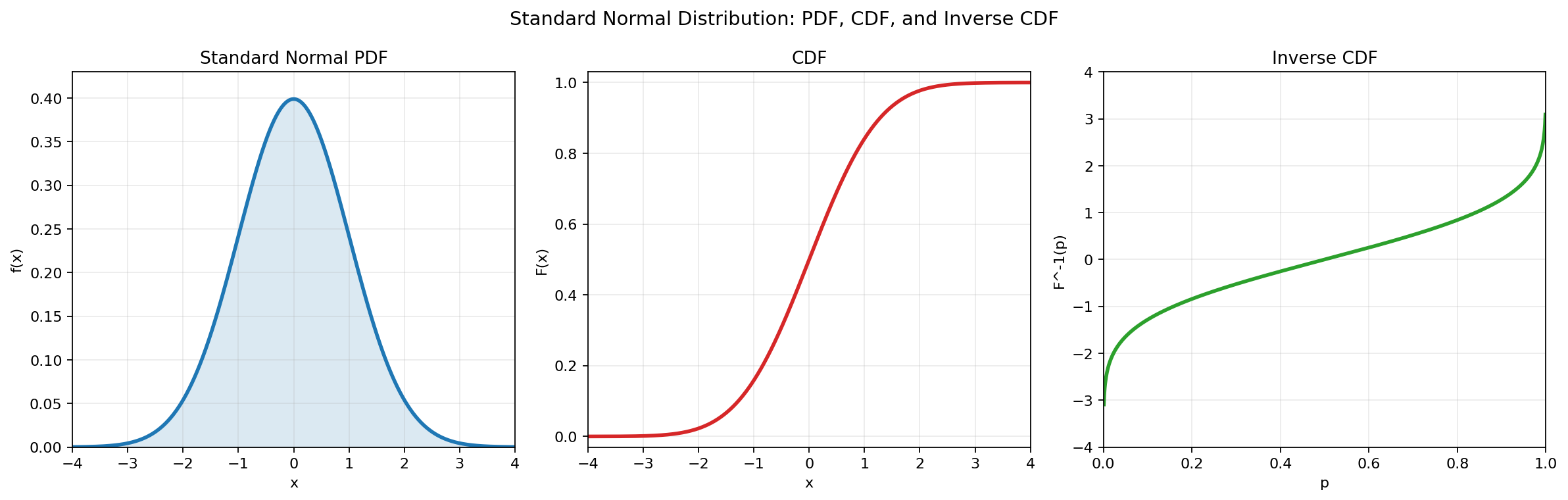
为了更直观地理解，我们可以看下面这张图。假设我们要生成服从标准正态分布的随机数：从左侧的 PDF 可以看出，标准正态分布的随机数绝大部分都密集分布在 $(-2, 2)$ 这个区间内，而而观察右侧的 CDF 反函数 $F^{-1}(u)$ 就会发现，当我们对横轴（即输入 $U$ ）在 $[0, 1]$ 上进行均匀抽样时，纵轴输出的 $X = F^{-1}(U)$ 绝大部分的几率都会落在 $(-2, 2)$ 区间内（因为只有在 $U$ 极度逼近 0 或 1 的边缘时， $X$ 才会飞向无穷大），正好满足正态分布

所以我们通常要使用服从在 $(0,1)$ 区间均匀分布的随机数来获得服从其他分布的随机数时可以遵循下面这个步骤：

让电脑生成一个 $0 \sim 1$ 的随机数 $u$
把 $u$ 带入该分布的 CDF 反函数 $F^{-1}(u)$ 中
得到的结果就是该分布的随机数

获得服从 Lambertian Diffuse Model 的 pdf 的采样#

根据上面的步骤生成随机数很简单，我们看看第二步应该做怎么做

我们的 pdf 是 $p(\omega) = \frac{\cos \theta}{\pi}$ ，它的自变量是一个立体角，我们需要找到立体角与实数的对应关系(因为我们的随机数是”实数”)，我们知道微分立体角与球坐标系下的角度的关系（我们一直使用单位球，因为我们讨论的是方向，而方向我们通常只使用单位向量）是

d\omega = \sin \theta d\theta d\phi

而我们知道球坐标系与直角坐标系的关系是

\left\{\begin{matrix} x =\sin\theta\cos\phi\\ y=\sin\theta\sin\phi \\ z=\cos\theta \end{matrix}\right.

而随机数（ $u_1, u_2 \sim U(0, 1)$ ）与角度（ $\theta, \phi$ ）之间的关系，由 CDF 反函数确定，我们唯一需要解决的问题就是如何将 $p(\omega) = \frac{\cos \theta}{\pi}$ 的自变量转换为 $\theta, \phi$

根据连续型多元随机变量的概率积分定义，总概率在不同坐标系下表达时应当保持恒等
所以

\iint p(\theta, \phi) \, d\theta \, d\phi = \int p(\omega) \, d\omega = \iint \left( \frac{\cos\theta}{\pi} \right) \sin\theta \, d\theta \, d\phi

由此，我们直接得到了关于 $\theta$ 和 $\phi$ 的联合概率密度函数

p(\theta, \phi) = \frac{1}{\pi} \cos\theta \sin\theta

而逆变换采样法在数学上是一个“一维定理”，它根本没办法直接处理多维的联合概率密度函数，所以我们需要将这个联合概率密度拆分为两个边缘概率密度

根据概率论对联合 PDF 的其中一个自变量在定义域上进行积分，就能得到另一个自变量的边缘概率密度函数

方位角 $\phi$ 的边缘 PDF
$\theta$ 的取值范围是半球的 $[0, \frac{\pi}{2}]$

p(\phi) = \int_{0}^{\frac{\pi}{2}} p(\theta, \phi) \, d\theta = \int_{0}^{\frac{\pi}{2}} \frac{1}{\pi} \cos\theta \sin\theta \, d\theta

凑微分有

p(\phi) = \frac{1}{\pi} \int_{0}^{\frac{\pi}{2}} \sin\theta \, d(\sin\theta) = \frac{1}{\pi} \left[ \frac{1}{2}\sin^2\theta \right]_0^{\frac{\pi}{2}} = \frac{1}{2\pi}

天顶角 $\theta$ 的边缘 PDF
$\phi$ 的取值范围是整个圆周的 $[0, 2\pi]$

p(\theta) = \int_{0}^{2\pi} p(\theta, \phi) \, d\phi = \int_{0}^{2\pi} \frac{1}{\pi} \cos\theta \sin\theta \, d\phi

p(\theta) = \frac{1}{\pi} \cos\theta \sin\theta \int_{0}^{2\pi} 1 \, d\phi = \frac{1}{\pi} \cos\theta \sin\theta \cdot 2\pi = 2\cos\theta \sin\theta

此时细心的你会发现，如果把我们求得的两个边缘 PDF 相乘

p(\theta) \cdot p(\phi) = (2\cos\theta \sin\theta) \cdot \left(\frac{1}{2\pi}\right) = \frac{1}{\pi} \cos\theta \sin\theta = p(\theta, \phi)

它们相乘的结果刚好等于联合 PDF！在概率论中，这严格证明了随机变量 $\theta$ 和 $\phi$ 是相互独立的。正因为独立，我们接下来可以放心地对它们各自单独使用一维的逆变换采样

呼，终于解决了前置问题终于可以使用逆变换采样法了

对 $p(\phi)$ 在 $[0, \phi]$ 积分得到其 CDF $F(\phi)$

F(\phi) = \int_{0}^{\phi} \frac{1}{2\pi} d\phi = \frac{\phi}{2\pi}

求反函数，我们令 $F(\phi)$ 的反函数为 $F^{-1}(u_1)$ ，我们令 $u_1 = F(\phi)$ 根据反函数的性质：

F^{-1}(F(\phi)) = \phi

F^{-1}(u_1) =\phi = 2\pi u_1

同理我们可以得到

\sin\theta = \sqrt{u_2}

我们没必要解出 $\theta = \arcsin(\sqrt{u_2})$ ，因为我们最终需要将其转化为直角坐标

再看我们的直角坐标与球坐标之间的转换关系

\left\{\begin{matrix} x =\sin\theta\cos\phi\\ y=\sin\theta\sin\phi \\ z=\cos\theta \end{matrix}\right.

其中 $\sin\theta$ 我们已经知道了， $\cos\phi,\sin\phi$ 我们也已经知道了为 $\cos (2\pi u_1),\sin (2\pi u_1)$
就差最后一个 $\cos\theta$ 了，这个也非常好算根据 $\sin^2\theta + \cos^2\theta = 1$ ，我们可以算出

\cos\theta = \sqrt{1 - u_2}

所以最终我们得到

\left\{\begin{matrix} x =\sqrt{u_2}\cdot \cos(2\pi u_1)\\ y=\sqrt{u_2}\cdot \sin(2\pi u_1) \\ z=\sqrt{1 - u_2} \end{matrix}\right.

所以根据上面的推导我们将代码改为

1
std::optional<Vec3> sample(const Vec3& wi, const Vec3& normal)
2
{
3
    Vec3 local_wo = sampleCosineWeightedHemisphere();
4
    Vec3 wo = toWorld(local_wo, normal);
5

6
    if (dot(normal, wo) <= 1e-6) {
7
        return std::nullopt;
8
    }
9

10
    return unitVector(wo);
11
}
12

13
static Vec3 sampleCosineWeightedHemisphere()
14
{
15
    const double u1 = math::randomDouble();
16
    const double u2 = math::randomDouble();
17

18
    const double phi = 2.0 * math::PI * u1;
19
    const double r = std::sqrt(u2);
20

21
    const double x = r * std::cos(phi);
22
    const double y = r * std::sin(phi);
23
    const double z = std::sqrt(std::max(0.0, 1.0 - u2));
24

25
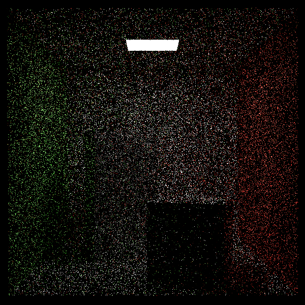
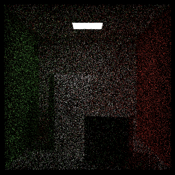
    return Vec3(x, y, z);
26
}

下面是在递归深度32，spp8下渲染出的两张图，上面这张是使用均匀采样，而下面那张是使用重要性采样，可以看出差距还是很明显的，尤其是在high box上

Implementing Russian Roulette#

在 Re0:0x02 中我们已经了解过了 Russian Roulette 的原理，这里我们来实现它。我们希望在实现 RR 的基础上保留最小的递归次数，防止光线刚开始生成就被RR杀死，由于是 RR 概率事件，所以有可能你的运气非常不好还是会进行多次递归，所以我们还需要保留最大递归次数，

所以我们修改一下常量，其中 kSurvivalProbability 是 RR 中光线的存活概率

1
    static constexpr int kMinDepth = 4;
2
    static constexpr int kMaxDepth = 128;
3
    static constexpr int kSamplesPerPixel = 8;
4
    static constexpr double kSurvivalProbability = 0.8;

由于在 RR 中我们需要对在 $[0,1)$ 上进行一个均匀采样，所以我们提供一个私有方法

1
double randomProbability() const
2
    {
3
        static thread_local std::mt19937 generator(std::random_device{}());
4
        static thread_local std::uniform_real_distribution<double> distribution(0.0, 1.0);
5
        return distribution(generator);
6
    }

然后我们实现我们的 RR traceRay 版本

1
Vec3 traceRay(const Ray& ray, const std::vector<std::unique_ptr<Object>>& objects)
2
    {
3
        return traceRay(ray, objects, 0);
4
    }
5

6
    Vec3 traceRay(const Ray& ray, const std::vector<std::unique_ptr<Object>>& objects, int depth)
7
    {
8
        if (depth >= kMaxDepth) {
9
            return Vec3(0.0, 0.0, 0.0);
10
        }
11

12
        bool hit_anything = false;
13
        bool is_light = false;
14
        double closest_t = std::numeric_limits<double>::max();
15
        InterInfo closest_info;
16
        std::shared_ptr<Material> material = nullptr;
17

18
        for (const auto& object : objects) {
19
            const InterInfo info = object->getInterInfo(ray);
20
            if (!info.is_Intersected || info.closest_t >= closest_t) {
21
                continue;
22
            }
23

24
            hit_anything = true;
25
            is_light = object->isLight();
26
            closest_t = info.closest_t;
27
            closest_info = info;
28
            material = object->getMaterial();
29
        }
30

31
        if (!hit_anything || !material) {
32
            return Vec3(0.0, 0.0, 0.0);
33
        }
34

35
        if (is_light) {
36
            return material->eval();
37
        }
38

39
        const Vec3 wo = -ray.getDirection();
40
        const Vec3 normal = faceForward(closest_info.normal, wo);
41

42
        const std::optional<Vec3> sampled_direction = material->sample(wo, normal);
43
        if (!sampled_direction.has_value()) {
44
            return Vec3(0.0, 0.0, 0.0);
45
        }
46

47
        const double sample_pdf = material->pdf(*sampled_direction, wo, normal);
48
        if (sample_pdf <= 1e-8) {
49
            return Vec3(0.0, 0.0, 0.0);
50
        }
51

52
        // 计算被积函数中的cos项
53
        const double cos_theta = std::max(0.0, dot(normal, *sampled_direction));
54

55
        // 获取反射后的光线
56
        const Ray scattered_ray(closest_info.position + normal * 1e-4, *sampled_direction);
57

58
        // 俄罗斯轮盘赌
59
        Vec3 incoming_light;
60
        if (depth < kMinDepth) {
61
            // 在达到最小深度前，强制继续追踪
62
            incoming_light = traceRay(scattered_ray, objects, depth + 1);
63
        } else {
64
            // 达到最小深度后，使用俄罗斯轮盘赌
65
            if (randomProbability() < kSurvivalProbability) {
66
                // 存活，继续追踪，并将贡献除以存活概率以保持无偏
67
                incoming_light = traceRay(scattered_ray, objects, depth + 1) / kSurvivalProbability;
68
            } else {
69
                // 终止，返回黑色
70
                incoming_light = Vec3(0.0, 0.0, 0.0);
71
            }
72
        }
73

74
        // 返回最终颜色
75
        return material->eval() * incoming_light * (cos_theta / sample_pdf);
76
    }

代码结构调整#

在 Re0:0x01 中，我们实现了一个非常简单的Path Tracing 渲染器，但是那个适合为了快速搭建出架构有许多设计不合理的地方，所以我们现在需要对其进行一些调整。
我们首先观察到代码中很多地方都在用到相似的数学功能，所以我们把这些整合到Re0Math.h中：

1
#pragma once
2
#include <random>
3

4
namespace math {
5
static double randomDouble(double min = 0.0, double max = 1.0)
6
{
7
    static thread_local std::mt19937 generator(std::random_device{}());
8
    std::uniform_real_distribution<double> distribution(min, max);
9
    return distribution(generator);
10
}
11

12
} // namespace math

这样 Renderer.h 中的randomProbability和 randomOffset 可以改为使用这个通用的函数了

我们再把 Material.h 中的 sampleUniformHemisphere、sampleCosineWeightedHemisphere和 toWorld 移到 Re0Math.h 中

我们再新建一个文件 Generator.h 专门为我们生成图片

1
#pragma once
2
#include "Vec3.h"
3

4
#include <cstdint>
5

6
#include <algorithm>
7
#include <fstream>
8
#include <string>
9
#include <vector>
10

11
class Generator {
12
public:
13
    Generator(std::string file_name, uint32_t width = 800, uint32_t height = 600)
14
        : m_file_name(file_name),
15
          m_image_width(width),
16
          m_image_height(height)
17
    {}
18

19
    void writePPM(const std::vector<Vec3>& data)
20
    {
21
        std::ofstream ofs(m_file_name, std::ios::binary);
22

23
        ofs << "P6\n" << m_image_width << " " << m_image_height << "\n255\n";
24

25
        for (int i = 0; i < m_image_width * m_image_height; ++i) {
26
            const unsigned char pixel[] = {
27
                static_cast<unsigned char>(toByte(data[i].x())),
28
                static_cast<unsigned char>(toByte(data[i].y())),
29
                static_cast<unsigned char>(toByte(data[i].z())),
30
            };
31
            ofs.write(reinterpret_cast<const char*>(pixel), 3);
32
        }
33

34
        ofs.close();
35
    }
36

37
    static void printProgress(int completed_rows, int total_rows)
38
    {
39
        const double progress = static_cast<double>(completed_rows) / total_rows;
40
        const int filled = static_cast<int>(progress * 40);
41

42
        std::cout << "\rRendering [";
43
        for (int i = 0; i < 40; ++i) {
44
            std::cout << (i < filled ? '#' : '-');
45
        }
46
        std::cout << "] " << static_cast<int>(progress * 100.0) << "%";
47

48
        if (completed_rows == total_rows) {
49
            std::cout << '\n';
50
        }
51
        std::cout << std::flush;
52
    }
53

54
    void setImageSize(uint32_t width, uint32_t height)
55
    {
56
        m_image_width = width;
57
        m_image_height = height;
58
    }
59

60
    void setFileName(const std::string& file_name)
61
    {
62
        m_file_name = file_name;
63
    }
64

65
private:
66
    int toByte(double value)
67
    {
68
        const double gamma_corrected = std::sqrt(std::clamp(value, 0.0, 1.0));
69
        return static_cast<int>(255.999 * gamma_corrected);
70
    }
71

72
    uint32_t m_image_width;
73
    uint32_t m_image_height;
74
    std::string m_file_name;
75
};

并将main改为

1
int main()
2
{
3
    const int width = 600;
4
    const int height = 600;
5

6
    Camera camera(width, height, Vec3(0.0, 0.0, -800.0), Vec3(0.0, 0.0, 280.0), Vec3(0.0, 1.0, 0.0), 40.0);
7

8
    Scene scene(camera);
9
    buildCornellBox(scene);
10

11
    Renderer renderer;
12
    renderer.render(scene.getCamera(), scene.getObjects());
13

14
    Generator generator("out22.ppm", width, height);
15
    generator.writePPM(scene.getCamera().getFrameBuffer());
16

17
    return 0;
18
}

并在 Renderer.h 中使用 Generator::printProgress

最后把 Renderer.h 中的 faceForward 移动到 Vec3.h 中

Implementing Light Sampling (Next Event Estimation)#

接下来我们实现对光源的采样简称NEE ，NEE 的渲染方程是这样：

L_o(x, \omega_o) = \int_{\mathcal{A_{light}} } f_r(x,\omega_i, \omega_o) L_i(x,\omega_i)V(x,x^{\prime}) \frac{\cos \theta_e \cos\theta_i}{||x-x^{\prime}||^2}dA

其中

V(x,x^{\prime}) = \left\{\begin{matrix} 1 & \text{如果} x\text{和}x^{\prime}\text{之间没有物体遮挡} \\ 0 & 否则 \end{matrix}\right.

其中 visibility 项我们可以在 shading point 上生成一条光线（Shadow Ray）连向光源，判断Shadow Ray在除了击中光源之外有没有击中其他物体，如果没有则返回1，否则返回0

所以就此我们可以将 Visibility 项去除看一定会击中光源的情况，此时渲染方程为：

L_o(x, \omega_o) = \int_{\mathcal{A_{light}} } f_r(x,\omega_i, \omega_o) L_i(x,\omega_i)\frac{\cos \theta_e \cos\theta_i}{||x-x^{\prime}||^2}dA

对应的 Monte Carlo 采样估计量为：

\hat{L}_o(p, \omega_o)=\frac{1}{N}\sum_{i=1}^N\frac{f_r(p,\omega_i,\omega_o)L_i(p,\omega_i)\cos \theta_e \cos\theta_i}{p_{pdf}(x^{\prime})\cdot ||x-x^{\prime}||^2}

这里唯一不知道的就是 pdf 和采样策略了，通常我们认为光源是均匀发光的并不会一些地方特别亮，一些地方又暗一些，所以我们直接使用随机均匀采样就行了，那么对应的 pdf 就是面积的均匀分布

所以 pdf 为：

p_{pdf}(x^{\prime}) = \frac{1}{A_{light}}

我们在实现中先使用简单的加权平均来合并 BRDF 采样和 NEE ，未来我们再实现 MIS

由于我们需要获取光源采样点的位置（计算距离），还需要计算 $\cos \theta_e$ ，以及 pdf 所以我们在 Object.h中 添加

1
struct LightSample {
2
    Vec3 position;
3
    Vec3 normal;
4
    double pdf;
5
};

并且给 Object 添加

1
virtual std::optional<LightSample> sampleLight() const
2
{
3
    return std::nullopt;
4
}
5

6
// 方便我们获取面积
7
virtual double getArea() const
8
{
9
    return 0.0;
10
}

然后我们给 Triangle.h 添加

1
std::optional<LightSample> sampleLight() const override
2
{
3
    double u1 = math::randomDouble();
4
    double u2 = math::randomDouble();
5

6
    if (u1 + u2 > 1.0) {
7
        u1 = 1.0 - u1;
8
        u2 = 1.0 - u2;
9
    }
10

11
    // 重心坐标获取三角形内部的点，Re0:0x01中介绍过
12
    Vec3 position = p1_ + u1 * (p2_ - p1_) + u2 * (p3_ - p1_);
13

14
    return LightSample{position, normal_, 1.0 / getArea()};
15
}
16

17
double getArea() const override
18
{
19
    return (cross((p2_ - p1_), (p3_ - p1_))).length() / 2.0;
20
}

对于 sphere.h

1
// 暂时不实现
2
std::optional<LightSample> sampleLight() const override
3
{
4
    return std::nullopt;
5
}
6

7
double getArea() const override
8
{
9
    return 4 * math::PI * radius_ * radius_;
10
}

由于我们的 NEE 对应的 Monte Carlo 估计量中有一个 $L_i$ 而这个我们没办法通过递归获取，所以我们给Material.h需要添加一个发光的 Radiance

1
Vec3 emission_ = 0.0;

以及

1
Vec3 emission() const
2
{
3
    return emission_;
4
}
5

6
void setEmission(const Vec3& emission)
7
{
8
    emission_ = emission;
9
}

并且修改main.cpp中的buildCornellBox

1
...
2
const std::shared_ptr<Material> white = std::make_shared<Material>(Vec3(0.725, 0.710, 0.680));
3
const std::shared_ptr<Material> red = std::make_shared<Material>(Vec3(0.630, 0.065, 0.050));
4
const std::shared_ptr<Material> green = std::make_shared<Material>(Vec3(0.140, 0.450, 0.091));
5
const std::shared_ptr<Material> light = std::make_shared<Material>(Vec3(0.0,0.0,0.0));
6
 light->setEmission(Vec3(15.0, 15.0, 15.0) * math::PI);
7
...

再修改Renderer.h中的traceRay中的

1
// 如果第一次递归就命中光源直接返回光源的emission，否则返回 0 避免与NEE 双算
2
 if (is_light) {
3
    return depth == 0 ? material->emission() : Vec3(0.0, 0.0, 0.0);
4
}

我们先给 Renderer.h 添加一个 Visibility 判断函数

1
bool visibleToLight(const Vec3& origin,
2
                    const Vec3& direction,
3
                    const double& max_distance,
4
                    const Object* light_object,
5
                    const std::vector<std::unique_ptr<Object>>& objects) const
6
{
7
    const Ray shadow_ray(origin, direction);
8

9
    for (const auto& object : objects) {
10
        const InterInfo info = object->getInterInfo(shadow_ray);
11
        if (!info.is_Intersected) {
12
            continue;
13
        }
14

15
        if (info.closest_t >= max_distance - 1e-4) {
16
            continue;
17
        }
18
        if (object.get() == light_object) {
19
            continue;
20
        }
21

22
        return false;
23
    }
24

25
    return true;
26
}

由于我们每次递归的适合需要对光源进行一次采样，所以我们需要提前知道光源是哪些物体所以我们添加一个成员变量保存

1
std::vector<Object*> lights_;

并提前找出所有光源

1
void prepareLights(const std::vector<std::unique_ptr<Object>>& objects)
2
{
3
    lights_.clear();
4
    for (const auto& object : objects) {
5
        if (object->isLight()) {
6
            lights_.push_back(object.get());
7
        }
8
    }
9
}

并在渲染前就调用

1
void render(Camera& camera, const std::vector<std::unique_ptr<Object>>& objects)
2
{
3
    prepareLights(objects);
4
...
5
}

最后我们给traceRay添加

1
Vec3 direct_light;
2
for (const auto& light : lights_) {
3
    const auto light_sample = light->lightSample();
4
    if (!light_sample.has_value()) {
5
        continue;
6
    }
7
    const Vec3 light_direction = light_sample->position - closest_info.position;
8
    const double distance_squared = light_direction.lengthSquared();
9
    const double distance = std::sqrt(distance_squared);
10

11
    const Vec3 wi = light_direction / distance;
12

13
    const double cos_i = std::max(0.0, dot(normal, wi));
14
    const double cos_e = std::max(0.0, dot(light_sample->normal, -wi));
15

16
    if (cos_i <= 0.0 || cos_e <= 0.0) {
17
        continue;
18
    }
19

20
    if (!visibleToLight(closest_info.position + normal * 1e-4, wi, distance, light, objects)) {
21
        continue;
22
    }
23

24
    const Vec3 Le = light->getMaterial()->emission();
25
    const Vec3 fr = material->eval();
26

27
    direct_light += Le * fr * cos_i * cos_e / (distance_squared * light_sample->pdf);
28
}

最后我们的Renderer.h如下

1
#pragma once
2
#include "Camera.h"
3
#include "Generator.h"
4
#include "Material.h"
5
#include "Object.h"
6
#include "Ray.h"
7
#include "Re0Math.h"
8
#include "Scene.h"
9
#include "Vec3.h"
10

11
#include <algorithm>
12
#include <iostream>
13
#include <limits>
14
#include <memory>
15
#include <optional>
16
#include <random>
17
#include <vector>
18

19
class Renderer {
20
public:
21
    Renderer() = default;
22
    ~Renderer() = default;
23

24
    void render(Camera& camera, const std::vector<std::unique_ptr<Object>>& objects)
25
    {
26
        prepareLights(objects);
27
        const int image_width = camera.getImageWidth();
28
        const int image_height = camera.getImageHeight();
29
        auto& frame_buffer = camera.getFrameBuffer();
30
        int completed_rows = 0;
31

32
        for (int j = 0; j < image_height; ++j) {
33
            for (int i = 0; i < image_width; ++i) {
34
                Vec3 pixel_color;
35
                for (int sample = 0; sample < kSamplesPerPixel; ++sample) {
36
                    const Ray ray = camera.getRay(i, j, math::randomDouble(-0.5, 0.5), math::randomDouble(-0.5, 0.5));
37
                    pixel_color += traceRay(ray, objects);
38
                }
39
                pixel_color /= kSamplesPerPixel;
40
                frame_buffer[j * image_width + i] = pixel_color;
41
            }
42
            ++completed_rows;
43
            Generator::printProgress(completed_rows, image_height);
44
        }
45

46
    }
47

48
private:
49
    static constexpr int kMinDepth = 4;
50
    static constexpr int kMaxDepth = 128;
51
    static constexpr int kSamplesPerPixel = 4;
52
    static constexpr double kSurvivalProbability = 0.8;
53

54
    std::vector<Object*> lights_;
55

56
    Vec3 traceRay(const Ray& ray, const std::vector<std::unique_ptr<Object>>& objects)
57
    {
58
        return traceRay(ray, objects, 0);
59
    }
60

61
    Vec3 traceRay(const Ray& ray, const std::vector<std::unique_ptr<Object>>& objects, int depth)
62
    {
63
        if (depth >= kMaxDepth) {
64
            return Vec3(0.0, 0.0, 0.0);
65
        }
66

67
        bool hit_anything = false;
68
        bool is_light = false;
69
        double closest_t = std::numeric_limits<double>::max();
70
        InterInfo closest_info;
71
        std::shared_ptr<Material> material = nullptr;
72

73
        for (const auto& object : objects) {
74
            const InterInfo info = object->getInterInfo(ray);
75
            if (!info.is_Intersected || info.closest_t >= closest_t) {
76
                continue;
77
            }
78

79
            hit_anything = true;
80
            is_light = object->isLight();
81
            closest_t = info.closest_t;
82
            closest_info = info;
83
            material = object->getMaterial();
84
        }
85

86
        if (!hit_anything || !material) {
87
            return Vec3(0.0, 0.0, 0.0);
88
        }
89

90
        if (is_light) {
91
            return depth == 0 ? material->emission() : Vec3(0.0, 0.0, 0.0);
92
        }
93

94
        const Vec3 wo = -ray.getDirection();
95
        const Vec3 normal = faceForward(closest_info.normal, wo);
96

97
        const std::optional<Vec3> sampled_direction = material->sample(wo, normal);
98
        if (!sampled_direction.has_value()) {
99
            return Vec3(0.0, 0.0, 0.0);
100
        }
101

102
        const double sample_pdf = material->pdf(*sampled_direction, wo, normal);
103
        if (sample_pdf <= 1e-8) {
104
            return Vec3(0.0, 0.0, 0.0);
105
        }
106

107
        const double cos_theta = std::max(0.0, dot(normal, *sampled_direction));
108

109
        const Ray scattered_ray(closest_info.position + normal * 1e-4, *sampled_direction);
110

111
        Vec3 incoming_light;
112

113
        if (depth < kMinDepth) {
114
            incoming_light = traceRay(scattered_ray, objects, depth + 1);
115
        } else {
116
            if (math::randomDouble() < kSurvivalProbability) {
117
                incoming_light = traceRay(scattered_ray, objects, depth + 1) / kSurvivalProbability;
118
            } else {
119
                incoming_light = Vec3(0.0, 0.0, 0.0);
120
            }
121
        }
122

123
        Vec3 direct_light;
124
        for (const auto& light : lights_) {
125
            const auto light_sample = light->lightSample();
126
            if (!light_sample.has_value()) {
127
                continue;
128
            }
129
            const Vec3 light_direction = light_sample->position - closest_info.position;
130
            const double distance_squared = light_direction.lengthSquared();
131
            const double distance = std::sqrt(distance_squared);
132

133
            const Vec3 wi = light_direction / distance;
134

135
            const double cos_i = std::max(0.0, dot(normal, wi));
136
            const double cos_e = std::max(0.0, dot(light_sample->normal, -wi));
137

138
            if (cos_i <= 0.0 || cos_e <= 0.0) {
139
                continue;
140
            }
141

142
            if (!visibleToLight(closest_info.position + normal * 1e-4, wi, distance, light, objects)) {
143
                continue;
144
            }
145

146
            const Vec3 Le = light->getMaterial()->emission();
147
            const Vec3 fr = material->eval();
148

149
            direct_light += Le * fr * cos_i * cos_e / (distance_squared * light_sample->pdf);
150
        }
151

152
        const Vec3 indirect_light = material->eval() * incoming_light * (cos_theta / sample_pdf);
153

154
        return direct_light + indirect_light;
155
    }
156

157
    bool visibleToLight(const Vec3& origin,
158
                        const Vec3& direction,
159
                        const double& max_distance,
160
                        const Object* light_object,
161
                        const std::vector<std::unique_ptr<Object>>& objects) const
162
    {
163
        const Ray shadow_ray(origin, direction);
164

165
        for (const auto& object : objects) {
166
            const InterInfo info = object->getInterInfo(shadow_ray);
167
            if (!info.is_Intersected) {
168
                continue;
169
            }
170

171
            if (info.closest_t >= max_distance - 1e-4) {
172
                continue;
173
            }
174
            if (object.get() == light_object) {
175
                continue;
176
            }
177

178
            return false;
179
        }
180

181
        return true;
182
    }
183

184
    void prepareLights(const std::vector<std::unique_ptr<Object>>& objects)
185
    {
186
        lights_.clear();
187
        for (const auto& object : objects) {
188
            if (object->isLight()) {
189
                lights_.push_back(object.get());
190
            }
191
        }
192
    }
193
};

最后我们在下面的参数下渲染出的对比图

1
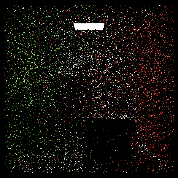
static constexpr int kMinDepth = 4;
2
static constexpr int kMaxDepth = 128;
3
static constexpr int kSamplesPerPixel = 4;
4
static constexpr double kSurvivalProbability = 0.8;

上面是 Without NEE 的结果，下面是 With NEE 的结果

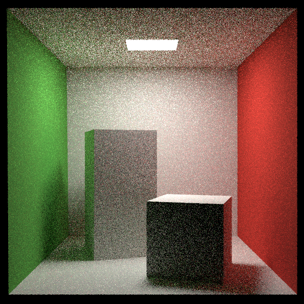
Implementing MIS#

还记得我们在Re0:0x02中提到的 Power Heuristic $\beta = 2$ MIS 吗？

我们需要计算

w_{BRDF} = \frac{p_{BRDF}^2(\omega_{BRDF})}{p_{BRDF}^2(\omega_{BRDF})+p_{\omega, Light}^2(\omega_{BRDF})}

w_{Light} = \frac{p_{\omega, Light}^2(\omega_{Light})}{p_{BRDF}^2(\omega_{Light})+p_{\omega, Light}^2(\omega_{Light})}

其中

p_{\omega, Light} = p_{Light} \cdot \frac{||x - x'||^2}{\cos \theta_e}

最后合并

L_o \approx w_{BRDF}L_{BRDF} + w_{Light}L_{Light}

我们先给Renderer.h添加一个

1
double powerHeuristic(const double pdf_a, const double pdf_b) const
2
{
3
    const double a2 = pdf_a * pdf_a;
4
    const double b2 = pdf_b * pdf_b;
5
    const double denominator = a2 + b2;
6
    if (denominator <= 0.0) {
7
        return 0.0;
8
    }
9

10
    return a2 / denominator;
11
}

对于 $w_{Light}$ 代码中我们已经有了所有的信息可以直接实现，但是对于 $w_{BRDF}$ 我们并不知道采样后生成的 scattered_ray 下一次是否会击中光源，如果没击中那么 $p_{\omega, Light}^2(\omega_{BRDF})$ 应该为0

所以我们需要调整一下我们的 traceRay，我们把上一次光线击中的物体 pdf 作为递归参数传递到下一次，这样我们就可以获取上一次物体的 pdf 和这一次击中光源时的 pdf 了

Q&A
Q：为什么可以使用上一次物体的pdf计算?
A：因为如果从 BRDF 采样这次击中了光源，说明这是最后一次递归了，上一次的Shading point是我们最后要算的 Shading point

1
Vec3 traceRay(const Ray& ray,
2
                const std::vector<std::unique_ptr<Object>>& objects,
3
                int depth,
4
                double previous_brdf_pdf)
5
{
6
    if (depth >= kMaxDepth) {
7
        return Vec3(0.0, 0.0, 0.0);
8
    }
9

10
    bool hit_anything = false;
11
    bool is_light = false;
12
    double closest_t = std::numeric_limits<double>::max();
13
    InterInfo closest_info;
14
    std::shared_ptr<Material> material = nullptr;
15
    Object* hit_object = nullptr;
16

17
    for (const auto& object : objects) {
18
        const InterInfo info = object->getInterInfo(ray);
19
        if (!info.is_Intersected || info.closest_t >= closest_t) {
20
            continue;
21
        }
22

23
        hit_anything = true;
24
        is_light = object->isLight();
25
        closest_t = info.closest_t;
26
        closest_info = info;
27
        material = object->getMaterial();
28
        hit_object = object.get();
29
    }
30

31
    if (!hit_anything || !material) {
32
        return Vec3(0.0, 0.0, 0.0);
33
    }
34

35
    if (is_light) {
36
        if (depth == 0) {
37
            return material->emission();
38
        }
39

40
        if (previous_brdf_pdf <= 1e-8 || !hit_object) {
41
            return Vec3(0.0, 0.0, 0.0);
42
        }
43

44
        const double light_area = hit_object->getArea();
45
        const double cos_e = std::max(0.0, dot(closest_info.normal, -ray.getDirection()));
46
        if (light_area <= 0.0 || cos_e <= 0.0) {
47
            return Vec3(0.0, 0.0, 0.0);
48
        }
49

50
        const double light_pdf = 1.0 / light_area;
51
        const double distance_squared = (closest_info.position - ray.getOrigin()).lengthSquared();
52
        const double solid_angle_light_pdf = light_pdf * distance_squared / cos_e;
53
        const double weight_brdf = powerHeuristic(previous_brdf_pdf, solid_angle_light_pdf);
54

55
        return weight_brdf * material->emission();
56
    }
57

58
    const Vec3 wo = -ray.getDirection();
59
    const Vec3 normal = faceForward(closest_info.normal, wo);
60

61
    const std::optional<Vec3> sampled_direction = material->sample(wo, normal);
62
    if (!sampled_direction.has_value()) {
63
        return Vec3(0.0, 0.0, 0.0);
64
    }
65

66
    const double brdf_pdf = material->pdf(*sampled_direction, wo, normal);
67
    if (brdf_pdf <= 1e-8) {
68
        return Vec3(0.0, 0.0, 0.0);
69
    }
70

71
    const double cos_theta = std::max(0.0, dot(normal, *sampled_direction));
72
    if (cos_theta <= 0.0) {
73
        return Vec3(0.0, 0.0, 0.0);
74
    }
75

76
    const Ray scattered_ray(closest_info.position + normal * 1e-4, *sampled_direction);
77

78
    Vec3 incoming_light;
79

80
    if (depth < kMinDepth) {
81
        incoming_light = traceRay(scattered_ray, objects, depth + 1, brdf_pdf);
82
    } else {
83
        if (math::randomDouble() < kSurvivalProbability) {
84
            incoming_light = traceRay(scattered_ray, objects, depth + 1, brdf_pdf) / kSurvivalProbability;
85
        } else {
86
            incoming_light = Vec3(0.0, 0.0, 0.0);
87
        }
88
    }
89

90
    Vec3 direct_light;
91
    for (const auto& light : lights_) {
92
        const auto light_sample = light->lightSample();
93
        if (!light_sample.has_value()) {
94
            continue;
95
        }
96
        const Vec3 light_direction = light_sample->position - closest_info.position;
97
        const double distance_squared = light_direction.lengthSquared();
98
        const double distance = std::sqrt(distance_squared);
99

100
        const Vec3 wi = light_direction / distance;
101

102
        const double cos_i = std::max(0.0, dot(normal, wi));
103
        const double cos_e = std::max(0.0, dot(light_sample->normal, -wi));
104

105
        if (cos_i <= 0.0 || cos_e <= 0.0) {
106
            continue;
107
        }
108

109
        if (!visibleToLight(closest_info.position + normal * 1e-4, wi, distance, light, objects)) {
110
            continue;
111
        }
112

113
        const Vec3 Le = light->getMaterial()->emission();
114
        const Vec3 fr = material->eval();
115
        const double light_pdf = light_sample->pdf * distance_squared / cos_e;
116
        const double brdf_pdf_to_light = material->pdf(wi, wo, normal);
117
        const double weight_light = powerHeuristic(light_pdf, brdf_pdf_to_light);
118

119
        direct_light += weight_light * Le * fr * (cos_i / light_pdf);
120
    }
121

122
    const Vec3 indirect_light = material->eval() * incoming_light * (cos_theta / brdf_pdf);
123

124
    return direct_light + indirect_light;
125
}

目前暂时只有 Lambertian 漫反射材质不好测试MIS的威力，等我们有了新的材质之后我们再测试

Shirone

背景#

The Lambertian Diffuse Model#

方向半球反射率#

推导#

Importance Sampling of the Lambertian Diffuse Model#

Cosine-Weighted Hemisphere Sampling#

逆变换采样法#

获得服从 Lambertian Diffuse Model 的 pdf 的采样#

Implementing Russian Roulette#

代码结构调整#

Implementing Light Sampling (Next Event Estimation)#

Implementing MIS#

Re0:PathTracing

继续阅读

换条路线

Shirone

背景#

The Lambertian Diffuse Model#

方向半球反射率#

推导#

Importance Sampling of the Lambertian Diffuse Model#

Cosine-Weighted Hemisphere Sampling#

逆变换采样法#

获得服从 Lambertian Diffuse Model 的 pdf 的采样#

Implementing Russian Roulette#

代码结构调整#

Implementing Light Sampling (Next Event Estimation)#

Implementing MIS#

分享文章

沿着主题读

换条路线